GIMP-LEVELS and GMIC : "drill-down"

first section:

I played on the same base image (which I post here, thanks to Issabella, it's one of her recent photos)



I got the same results, either applying the gimp_levels command or the GMIC commands you mentioned, let's see



here I used the single gimp_levels command with the following parameters: 40,215,0.7 to specify: shift right input black point to 40, shift left input white point to 215, set mean value to 0.7



here I used the following commands:
-cut 40,215 (same as in gimp)
-normalize 0,255
-apply_gamma 0.49 (I found this one correspondinf to the gimp value 0.7)


(continuing on next posts)

only a little summary comment on this first section:
- it seems that GIMP -in this functionality- is more synthetic that GMIC (which is unusual!)
one GIMP command vs three GMIC commands

I guess it could be nice to provide a native command to GMIC (like: gmic_gimp_levels)
to perform all the steps together

(continuing on next posts)

second section:

considering the use of gimp_levels (or corresponding gmic commands) I want to extend the area of problems related to its usage inside a filter.
Because:
-interactively, you may see very well "de visu" when an image requires modifications to the black-mid-white points, and play with the sliders (or parameters in gmic) until you get the desired result. But...
-inside a filter, you need a way to understand which could be the best values for them
Well, for the mean, it is quite easy (you may prefer a different value from the one detected for instance with the variable im in gmic).
The minimum and the maximum, viceversa, can not rely on the variables im and iM, because you may just have a single pixel having 0 value and im will be 0, idem for the 255 value.
In fact, applying both the gimp_normalize or the gmic_normalize you get a totally unchanged outcome, in those cases.
What is interesting for the human eye, is detecting whether there are enough black values and enough white values to appreciate the contrast.
In gimp I use the histogram command (in a loop) to set for instance the black values to a minimum of 1% of the pixels, the same for the white.
Which is the best equivalent in gmic to detect at which point should the black (and respectively the white) point be set to get -let's say- a 1% of pixels?

(continuing later on)

to complete my second section

taking always the same image as input
(it has NOT 0 as minimum value, but 10, so something is changed using normalize command(s));
either using gimp normalize or gmic normalize I get:



but if I use my "special" normalize which set a minimum of 1% black + 1% white I get:



thus, I would like to perform the same using only gmic command(s)


another note:

in gimp levels there is a buttom "auto" which provides a better output than a standard gimp normalize; I don't know what it does, specifically, but is could be nice to have a kind of "auto" option also in gmic normalize

here the output of gimp "auto" levels

new attempt still playing on each channel

Good evening, dinasset
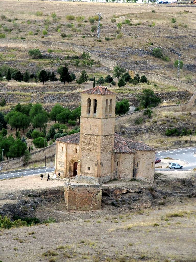
Thanks be to Issabella, for furnishing such an interesting image. The building seems precariously situated. Am I correct that the foreground is a dried lake/seabed? It reminds me of the ruined monasteries that dot the countryside of Erie and the United Kingdom, once beautiful buildings gone to ruin. In particular, Tintern Abbey in Wales, a beautiful, somber, bittersweet place.
On to business -
First, I think the thread has become misnamed. The questions are no longer small, and the answers certainly are not! This post, in fact, has become something like 3,000 words, so it will likely go into Beginners Cookbook at G'MIC Sourceforge in the fullness of time.
Second - I'd like to drill down on the term "gamma" as it is used with the Adjust Color Levels dialogue. In particular, the usage as inferred from this sentence in your post #16:

Particular Distinctions
The particular notion that I wish to dispel is that "blackpoint" is equivalent to G'MIC's "im", "gamma" is equivalent to G'MIC's "ia" and "whitepoint" is equivalent to 'iM"
Such is not the case. They constitute two sets of terms, each fulfilling different purposes.

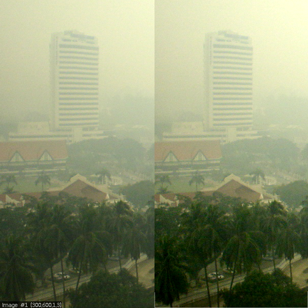
1. im, ia, and iM are statistical indicators concerning, in particular, the last item on an image list. G'MIC computes these at the behest of a -print command by visiting every pixel in an image and finding the smallest, largest and average value of the ensemble. I can direct G'MIC to tabulate these data for Issabella's image (IMG_1730.JPG) and report on them via "$ gmic -input IMG_1730.JPG -print" and will be told, among other things, that the minimum pixel intensity value found in this image across three channels is 10, ("im") the maximum intensity value found is 255 ("iM") and the mean (average) value is 137.543 ("ia"). These are observable statistical properties of image.
2. The values associated with "blackpoint", "gamma", and "whitepoint" are arguments that, when plugged into the computational engine that implements the "Input Level" slider, produces what I call a transfer function. They are arguments which can be chosen at whim, though one usually has some reason to choose particular values because of particular trends seen in image statistics. These reasons are driven as much by individual notions and heuristics. There is no invariant formula that I'm aware of that furnishes "correct" values for these arguments, based on some statistical ensemble of an image.

Blackpoints, Whitepoints and Gamma
Transfer functions may be applied to any number of images and have no association with any particular image. And while "blackpoint" and "whitepoint" are numeric quantities measurable in terms of pixel intensity, and, as such, are “of a kind” with "im", "ia," and "iM", they do not have the same meaning as these quantities. They serve purposes different than the expression of minimum or maximum values of particular images.
In devising transfer functions, "blackpoint" and "whitepoint" peg – or define – the two end point values of an intensity curve plotted on a graph that has horizontal and vertical scales, each graduated in the intensity values that unsigned eight bit integers are capable of expressing: the range [0,...255]. The curve is a literal visualization of a transfer function.
By themselves, "blackpoint" and "whitepoint" can only define very simple line-like (linear) transfer functions. The third ingredient, “gamma”, enables the generation of very versatile non-linear transfer functions, but before I take up the subject of this third ingredient, I want to spend a little bit of time with the concept of the transfer function itself – how it works and what it “means.” For that end, I only need the two “essential ingredients”, “whitepoint” and “blackpoint”.
Linear transfer functions
Now, it so happens that you have seen about a bazillon and seven of these things, give or take about five or six. Every time you bring up Gimp's Curve tool you see at least one transfer function, and can see as many as four per RGBA image, one for each channel.
The mechanism of these transfer functions is very simple.

• The horizontal scale represents operands from the set of intensities [0,...255]. You might consider them to be the set of intensities from a particular image, say the red channel of IMG_1730.JPG, but that is your interpretation, and is not intrinsic to the operands, for here in Brooklyn New York, I might be at the very same moment regarding them as the set of intensities from the gray scale image grayscale_16.png, and Ronounours in Caen may have yet a third image in mind. This transfer function exists independently of all of us, and the various interpretations that we might impose.
  
• The curve itself is an operator. It maps operands to resultants, here another set of intensities from the set [0,...255].
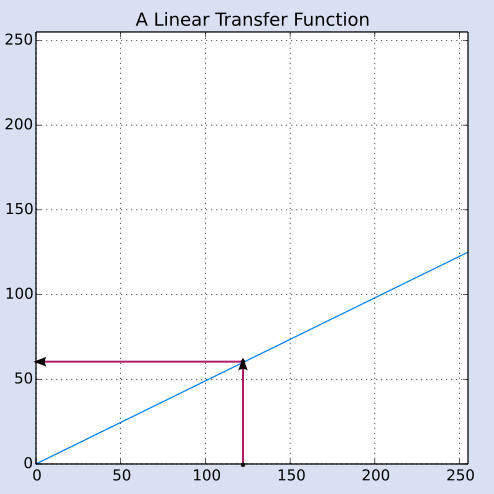
• The mechanism of operation entails choosing an operand, say “128” (mid gray), tracing vertically up until we encounter a point on the operator, inducing us to travel horizontally to the left until we encounter the vertical scale where we stop upon a resultant.
  
• Now for some particulars. Suppose for this particular transfer function, the “blackpoint” is zero, and the “whitepoint” is 125, which suffices to establish a simple linear transfer function. Then in this particular example, our resultant is 62.745, since this particular linear transfer function simply reduces operands by the ratio of 125/255, and 128 times 0.490196078 (125/255 in decimal) is 62.745.

That is the gist of how a transfer function works. It is a map from the operand grays to the resultant grays. This particular transfer function, or map, as you probably surmise, would be good for taking images that depict bright sunny scenes and turning them into versions lit by moonlight, darker, somber scenes. That said, I cannot stress enough that this particular usage has nothing to do with how we composed the original map. The “whitepoint” and “blackpoint” values do not have anything to do with particular images, or values like “im” or “iM” that might be discovered in particular images.
Gamma
Linear transfer functions, those simply composed from pegging white and black points, are useful in a limited sort of way, but do not adequately perform most of the mappings that photographers routinely require. Photographers routinely want to “stretch shadows” or “compress highlights” or desire “middle grays” to be darker or lighter than in the images they have in hand. These all call for non-linear mappings, that is, transfers from operands to resultants that cannot be adequately described by straight lines connecting the white and black points. The gamma value may not be essential for constructing transfer functions, but it is practically called for in most “real world” circumstances.
Black and white points are pixel intensities that peg particular operands to resultants. Doing such on two points on the graph allows a ratio to be established which scales operands linearly into resultants. Blackpoint matches up operand value zero to a resultant value, and necessarily is a pixel intensity. Similarly, Whitepoint matches up operand value 255 to another resultant value and is also necessarily a pixel intensity. Together these fix new intensity ranges for the resultant values. The appropriate range of values for both black and white points is [0,...255].
Gamma is intrinsically different from black and white points. It is not a pixel intensity, but a unitless number, a value that just “is” and one not representing a physical quantity. Thus, speaking of a gamma value as being equal to the average intensity of an image channel, “ia,” is a nonsense expression, akin to saying that an object is blue shaped.
When transfer functions are linear, the gamma value A. K. A. C2, is necessarily equal to one and is the midpoint of a relative logarithmic scale that ranges from (0,...10], the set from which gamma values are drawn.
You can observe the logarithmic behavior of gamma as you manipulate the middle slider of the Input Level control. You find it at its default value of 1.0. Pull it right (toward “white”) and it ranges toward (but never includes!) zero. In fact, it stops at 0.10. The image, meanwhile, exhibits stretched shadows and compressed highlights and, on average, becomes very dark. In contrast, pulling the control left (toward “black”) involves a rapid increase of numbers toward the value 10. Truly, this odd scale permits high precision for setting gamma values in the range of one to (nearly!) zero, but allows only coarse settings in the range of one to ten. The image, meanwhile, exhibits compressed shadows and stretched highlights and, on average, becomes very light.
Much of this behavior stems from how Gimp defines the transfer function, repeated here from the previous post:
(1.0)
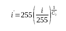
In particular, Gimp takes the reciprocal of the middle slider, C2, and uses that as the exponent of a power function. Pull the slider left, and the gamma value becomes less than one, the reciprocal becomes greater than one, and the mapping of operand values i to resultants i' follows a curve that bows down toward the southeast at degrees increasingly extreme as the slider approaches zero. Conversely, pulling the slider right sends the gamma value greater than one, the reciprocal goes less than one, and the mapping of operands to resultants follows a curve that bows up toward the northeast at degrees increasingly extreme as the slider approaches ten.
Clearly, if this argument becomes zero, then we will be dividing by zero in the exponent, Gimp will crash and Mitch Natterer will get rude email, which he does not want. So, to allow Mitch to sleep at night, gamma values may approach, but never be zero. Thus, the set of numbers from which we may choose gamma is open at one end; the elements of the set approach, but do not include zero.
The Adjust Color Levels tool has a nice big button that generates curves to effect its settings, transferring focus to Gimp's Color Curve tool. The Adjust Color Levels tool is essentially an alternate “front-end” to the Curve tool, one couched in terms more meaningful to photographers, but every tranform it performs may be alternately expressed by the Curve tool, though perhaps not as easily. It is not uncommon to refine the initial transfer functions produced by the Adjust Color Levels with the Curve tool.
The Emulation Pipeline
As I noted in the previous post, three G'MIC commands emulate the Color Adjust Levels dialog box. They do so by working in sequence through the following pipeline:

You transcribe the five values C1 – C5 from the Input and Output Level sliders, as depicted in my previous post, and that creates a pipeline that remaps the intensity levels in 'changeme.png' in a manner identical to the settings from the Color Adjust Levels dialog box.
The remapping takes place in stages. First, the -cut command sets all operand values less than <C1> to C1, sets all operand values greater than C3 to C3 but otherwise leaves operands alone.
Second, a -normalize command rescales the truncated range back to [0,...255], producing a simple linear transfer function that, when graphed, starts at coordinate point (C1, 0), the “blackpoint”, and ends at (C3, 255), the “whitepoint.
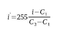
At this stage, the transfer function is functional, but limited, as it just rescales operand values to resultants. In particular, operands equal to C1 map to resultant zero, operands equal to C3 map to resultant 255, and all other operands i map to resultants i' by the relationship:
((2.0)
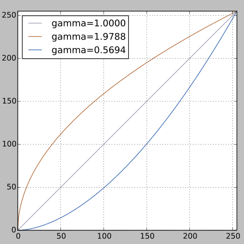
Third, -apply_gamma changes the mapping to a nonlinear one. There are two distinct outcomes, one distinguished by gamma values less than one, bending the curve “southeast,” the other distinguished by gamma values greater than one, bending the curve “northwest.” The first ( gamma=0.5694 ) produces a darker resultant scale, the second (gamma=1.9788) a lighter scale. In both cases, the progression of dark to light has been altered from a constant progression to a variable one that emphasizes either highlights or shadows.

Fourth, C4 and C5 together renormalize the range of the output to something other than the full range.
This graph summarizes how the various settings in the Color Adjust Levels transform from the initial identity transform, where operands map unchanged to resultants, to one that alters the appearance of an image.

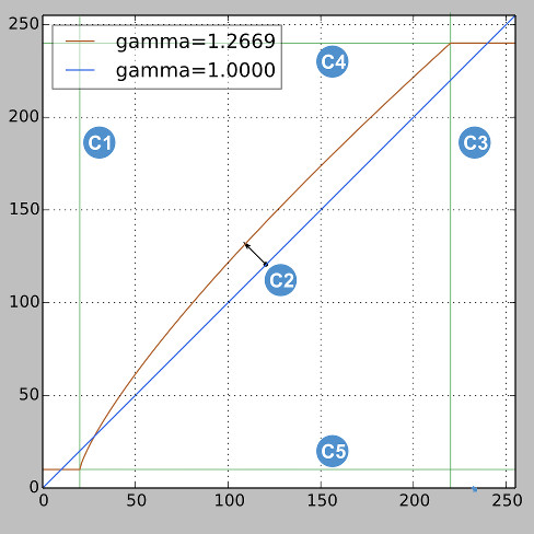
From this, it is clear that C2 is the most remarkable argument of the five, in that it neither scales nor cuts the curve, but instead controls the characteristics of a power function. It is also along among the five in that it is not a pixel measure, and this makes its behavior difficult to relate to an image. We know that when it equals one, the transfer function is linear. Otherwise it is a nonlinear function that, roughly alters highlights and shadows at different rates. It is not intuitive what an apt setting of this parameter might be if one had the shape of a particular transfer function in mind.
A Better Emulation Pipeline
Having the shape of a particular transfer function in mind suggests a solution to the singular parameter, gamma. There is the old bromide that three points not on a line suffices to define at least a degree two curve.
So instead of stumbling around for apt values of gamma, the approach that suggests itself is to solve for gamma using quantities that are more intuitively accessible – pixel measures. The idea is to define a gray that the midpoint of the transfer function should pass through, so that the curve starts at the blackpoint, proceeds through the midpoint positioned at some desired gray, and then finishes at the white point.
The scheme is not hard to implement. Regarding the power relation in which C2 is used to compute the resultant (2.0, above), we can adapt it to solve for C2, since we know the operand gray level (i) and we have declared the resultant gray, i' by fiat to be a particular value. We basically turn the relation around, using standard logarithmic identities that I first slept through in high school algebra.

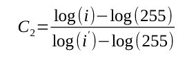
Unless you insist, I'll skip the algebraic to-ing and fro-ing that got C2 nestled in isolation on the left hand side, and with known (or declared by fiat) quantities on the right hand. Not surprisingly, should i = i', C2 reduces to one, which describes a linear transfer function. Otherwise, we generally choose i, the operand middle gray, to be equal to 128 and set i' to be the gray we would like to have in the translation from operands to resultants. Generally, to darken, choose i' so that i > i'; reverse the inequality to lighten. One is not restricted to using middle grays; if one is particular about a particular change in the shadow or highlights, a reference value of 80 or 210 for operand i is not out of the question. The signal advantage of choosing from the middle of the curve is generally a smoother transfer function.
Rather than plugging in numbers by fiat, it is worth our while to clean up our scripting act by defining a G'MIC function to package the mechanics. Here's one approach:

Copy it to your .gmic file ($HOME/.gmic, UNIX-like, %APPDATA%/gmic and then relaunch your G'MIC plug-in.
If, after contemplating some image such as , your eye tells you that a transfer function ought to start at a blackpoint of 10, pass through 90 at operand value 128, and stop at a whitepoint of 230, and you would prefer that the final image be normalized between 15, and 250, you would write:

Thus, instead of trying to decide on a particular gamma value, you give -leveladjust a midpoint gray observed in the given operand image ("current") and follow it with what level that gray should be in the resultant image ("target"), and the command will find the appropriate gamma value and apply it in conjunction with the other parameters.
Histogrammery
Deciding what best to do with an image in a script is probably a topic for another day. The G'MIC -histogram command will convert an image into another image with a depth of one row and a width of however many histogram bins that you want to segment the counts into. You can limit the -histogram count to specific ranges like the lowest 10% of an image's dynamic range (or some range in the middle). Each pixel in the converted image contains counts of pixels observed in the original image that are at particular gray levels.
What might be done with that data is often a matter of taste. It is one thing to run a script over a set of images because they are out of gamut according to some ICC profile; profiles contain hard numbers upon which to base adjustments. Matters of taste are more difficult to encode.
Take care
Garry

Garry, your answers are just awesome

Hi Garry.
Thanks a lot for your lesson in graphics/mathematics.
It seems that you take the opportunity from my "street-man oriented" "simple(?)" questions
(where the street is gimp+gmic image manipulation area) to write a nice set of tutorial pages
for a complete user manual for G'MIC. Good! David and many G'MIC coders/users will appreciate
your encyclopaedia (may we call it at the end Garry-pedia?).
But let me stay on my preferred Caesar's style, thus I synthetize what I got from you in a Q-A
scheme.

Q1: "which is the best command (or list of commands) in G'MIC to perform the colour manipulations
available in GIMP-LEVELS??
There you may "move" the 3 magical "points" (black - mean - white) -not only manually but also using
the corresponding command (gimp-levels) in script-fu.
Let's consider just the mean (the "ia" in GMIC); how can we "move" it either towards black or
towards white when needed such that all values between "im"(minimum value) and "ia" are "normalized"
between 0 and USER-MEAN-GOAL and values between "ia" and "iM"(maximum value) are "normalized"
between USER-MEAN-GOAL and 255?"

I reported my complete sentence because I like to underline that:
- I didn't say that im = black point, iM = white point
- I simply associated the mean with ia only to set our attention to the centre of the image values
to introduce the subsequent question ("how can...")
If we read slowly the question it appears evident that my goal was to have the command(s) to perform
what is performed in Gimp by the single commmand "gimp-levels", i.e.:
- move the im point (the minimum value) to 0 (black)
- move the iM point (the maximum value) to 255 (white)
(there two "moves" can perform the "stretching" of the values, if and only if im is NOT already 0 and iM is NOT already 255, point discussed in a subsequent post concerning the "normalize" function)
- change the mid value from im to the USER-MEAN-GOAL
(this will either stretch the dark values AND at the same time compress the light values or viceversa
depending of the difference between current im and desired im)

A1: you didn't answer immediately because you wanted me engaged in your "challenge": fine, I accepted
your point and tried to do my first attempts to enhance(?) that image
Later you provided me the analytical answer explaining in details what normalize, cut, and gamma commands
do in G'MIC. Good, I played with those and entered the subsequent series of observations/questions.
I could verify personally how those three commands can be used to get the result normally obtained by
the gimp-level function. Excellent! Thanks!
A great part of my subsequent posts are occupied by the sample images (using a very attractive original
image from Issabella).
Then came the note (let me assimilate it to a question, not to use another prefix...)

Q2: "only a little summary comment on this first section:
- it seems that GIMP -in this functionality- is more synthetic that GMIC (which is unusual!)
one GIMP command vs three GMIC commands.
I guess it could be nice to provide a native command to GMIC (like: gmic_gimp_levels)
to perform all the steps together"

A2: the last part of your last post gives the solution: you wrote that synthetic command to
"simulate" what gimp-levels performs. Excellent! I hope David will put it into the next update
of G'MIC filter. For the moment I will certainly put it in my directory. Thanks a lot.

Q3: "What is interesting for the human eye, is detecting whether there are enough black values and enough
white values to appreciate the contrast.
In gimp I use the histogram command (in a loop) to set for instance the black values to a minimum of 1%
of the pixels, the same for the white.
Which is the best equivalent in gmic to detect at which point should the black (and respectively the white)
point be set to get -let's say- a 1% of pixels?"

A3: "Deciding what best to do with an image in a script is probably a topic for another day.
The G'MIC -histogram command will convert an image into another image with a depth of one row and
a width of however many histogram bins that you want to segment the counts into.
You can limit the -histogram count to specific ranges like the lowest 10% of an image's dynamic range
(or some range in the middle).
Each pixel in the converted image contains counts of pixels observed in the original image that are
at particular gray levels."
OK, you got precisely what I need, the possibility to "count" only the pixels with a certain range of values
and change the value distribution until a count corresponding to the USER-GOAL is reached
(in my gimp only script the goal is set by default to 1% of black values and 1% of white values,
but the user can set the goal he/she likes).
Thus, I'm anxious to read your next post about that. Thanks.

Q4: "in gimp levels there is a buttom "auto" which provides a better output than a standard gimp normalize;
I don't know what it does, specifically, but is could be nice to have a kind of "auto" option
also in gmic normalize"

A4: open

To conclude: thanks, thanks, thanks.
I'm quite sure that other users/coders will benefit of your exhaustive explanations.

@okyl168: Thank you for your contribution to "Clearing Kuala Lumpur", the contest with no rules, no judges, and no prizes. But, at least, I'm enjoying all the variations that are being posted!

@Ronounours: Thank you David. And on random, incidental occasions, my answers happen to match the questions that the good, patient dinasset asks. I suppose to him my answers are like boxes of Cracker Jacks. You never know, but there might be a prize in one of them.

@dinasset: Gather ye, picture metrics.
Let's see how closely I can remain focussed on Question 3.
I'll use Issabella's fine picture, IMG_1730.JPG, venerable architecture in precarious circumstances.
Since the question involves 'darkest', 'lightest' 'average', I'm going to make a new version of IMG_1730.JPG containing computed luminance values of the RGB picture values, just to shrink the dataset a bit. Also note, in the code sections, I've placed single quotes around math sections (in curly braces: {}) and terminated lines with a backslash. (\). This is for cutting-and-pasting into bash shells, a kind of command shell popular on Linux machines. If you incorporate this code into a script, remove the single quotes and backslashes.
So! To begin:

The last bit sets a variable, onepct to the pixel count constituting one percent of a 768 by 1024 pixel grayscale image, an amount that is currently 7,864 pixels here in Brooklyn, New York. Well, 7,864 isn't exactly one percent because int() rounds its argument down to the nearest whole integer, but let's not quibble over a pixel or two precision. Spend some time with pages 11 and 12 of the gmic_reference.pdf document, where all of these substitution rules -- like @{-1,#} -- are enumerated in Ronounour's terse, but charming, Caesar-like prose (section 1.7).
This variable, onepct, is the width of a one pixel high "window" that I'm going to insert and move around in a data buffer. The data buffer contains all the pixels in the luminance version of Issabella's image, sorted in dark to light order.
To get this magical buffer, add the following bit of code to that above:

The echoing of 'drkave' should give you a value of 46.0305624789064. That is to say, the darkest 7,864 pixels of the luminance version of Issabella's image (pretty darn close to 1%) have an average intensity of 46.03 and change. Now, having spent some time with page 11 and 12 of the reference manual, you can easily modify the snippet above to report other metrics:
minimum: 11.23923492431641 @{-1,m}
maximum: 54.01943588256836 @{-1,M}
intensity of the 67th darkest pixel in the image: 21.98589515686035 @{-1,(66,0,0,0)} (66? Yes, for these buffers are zero-referenced, so the first item is indexed by 0 and the 67th item by 66)
What makes this assessment possible is, first, sort, which rearranges all the pixels of an image in dark-to-light order. second, shared, which creates a 'virtual image' comprised of the image buffer of its argument. How it's used is tedious to explain; fortunately, I've already explained it, so get ye to the gmic tutorial pages:

The key point here is that G'MIC treats this shared buffer as if it were an image in its own right, so it automagically computes the standard metrics on this 7,864 pixel buffer, the lowest one percent slice of a 786,432 buffer containing all of the pixels in the luminance version of Issabella's image, arranged from dark to light order.
How about the corresponding average of the 7,864 whitest pixels?

So here in Brooklyn, Noo Yawk, the weather is a fair, early Fall day and it so happens that the 7,864 lightest pixels in Issabella's image is 212.61 plus some change.
What's the average of the middle ten percent?

I get 141.754 and change.
So we're on a roll. How about averages on each ten percent segment?

These are the data I get:

Slice:0
Minimum: 11.23923492431641
Average: 75.48387111303468
Maximum: 95.31819152832031
Slice: 1
Minimum: 95.31819152832031
Average: 106.803287930142
Maximum: 116.0749435424805
Slice: 2
Minimum: 116.0749435424805
Average: 122.4229071395794
Maximum: 128.0794219970703
Slice: 3
Minimum: 128.0794219970703
Average: 132.9479761777032
Maximum: 137.4864349365234
Slice: 4
Minimum: 137.4864349365234
Average: 141.7539806978111
Maximum: 145.8587036132812
Slice: 5
Minimum: 145.8587036132812
Average: 149.3086186915349
Maximum: 152.7131042480469
Slice: 6
Minimum: 152.7131042480469
Average: 155.5979172468101
Maximum: 158.3314056396484
Slice: 7
Minimum: 158.3314056396484
Average: 161.3782763247584
Maximum: 164.4602661132812
Slice: 8
Minimum: 164.4602661132812
Average: 168.896755425723
Maximum: 174.0695495605469
Slice: 9
Minimum: 174.0695495605469
Average: 186.4907443977543
Maximum: 252.9277648925781

Let's edit the picture, shall we? It is our Profound and Omniscient Opinion (POOp) that Issabella's picture is running a little off Perfection. Perhaps We Are Full of That Which Is Animal Derived Garden Fertilizer, But Howsomeeveritshallbee, Perfection (we declare) means that any slip-sliding away from blackpoint, falling short of white point, or not having the average pixels cluster around middle gray (128) Is Just Not Right.
For the following, you'll need -leveladjust in your local gmic repository: $HOME/.gmic for Unix-like, or %APPDATA%/gmic for Windows


Run it:

Before

fixed:

Here's how leveladjust was set up and the gamma it used.
blackpoint: 46.0305624789064
current: 141.753980697811
target: 128
gamma: 0.8519184090548653
blackpoint: 212.6116803344851'

So, your correction on this was, I (think) I recall blackpoint 40, gamma 0.7, and whitepoint 215, no ?
In any case, both seem close to what Gimp's auto does.

How about Kuala Lumpur?


blackpoint: 39.34251697165379
current: 112.8168382014733
target: 128
gamma: 1.183195827301516
whitepoint: 173.9449747551812

That cuts the haze in the background but leaves the picture more-or-less in its original form, a deft touch.

So are these better? I dunno. It's based on a heuristic, and one person's heuristic is another person's haw, haw, haw. Better or worse, it is based on the idea of setting the black point to the average value of the lowest 1% count of pixels, the white point to the average value of the highest 1% count of pixels, and the gamma derived from a midpoint grey shift from whatever the average value of the middle 10% count of pixels is to the target value of 128. You tell me if that is better.
So that's your toy for the day. Probably too late for you to play with it, but there is always the morrow.

Take care,

Garry

wow! wow! wow!

that's my desired toy to work with! I'm feeling as an happy young boy (in spite of my very old age).
I did already some experiments, and I tell you my first impression:
- it works fine on images like the one used so far (Issabella's), that is: light images (ia>127)
- it generates too light images if the base original image is dark (ia<64)

I will play a lot to see whether I can find a possible modification to the filter, to become more "generalized".
If so, I will tell you

anyhow: really thanks a lot!
(and, last not least: your last post was written in a "language" fully understandable even by me, not a mathematician...)

addendum:
temporarily I found a way to have the filter more "generalized", i.e.
- setting the "goal" average not to 128 but to half a way between 128 and the current average

newave=($midave+128)/2
-leveladjust[-1] {$drkave},{$midave},{$newave},{$liteave},0,255 #Diego

this preserves better (imo) the characteristics of the original image
I guess (and hope) you'll find a much better mathematical solution (the gamma seems to be the problem)

Good day, dinasset:

Seems one of those rare days when my answer happens to match your question.

Apropos to my closing remark, -fixit probably needs to have an argument list, because its workings are based on assumptions that may not hold across all images. I think it very likely that the one gray presently fixed at 128, one of the two grays from which gamma is internally calculated, needs to be a parameter which one can choose. Here's the modification:

I adjusted the documentation to be more in keeping with G'MIC style. Additional parameters which suggest themselves could adjust the sampling ranges of $drkave, $midave and $lightave, presently 1%, 10%, and 1%, though it is not clear to me at present if the additonal to-ing and fro-ing involved would actually help or just be so much handwaving. I see you have been publishing some Scheme scripts for Gimp, which look like a bit of fun, and perhaps, with a representative example in front of you, you could experiment with adding or modifying parameters. I have a busy day today, but will check in from time to time.
Have fun and take care.
Garry

Even though this language is away beyond me, it looks like you guys sure know what you are doing. I get lost before I even reach the second line.

KUDO's guys.

Thanks Garry, your proposal is also to be taken into consideration, but in general I don' like letting the user making mistakes; so, in the case of the new target mean setted by the user I would prefer -if possible- that the check on that parameter allow only a value between current-value and 127.
(For example: if an image is dark, a value of 127 gives already almost bad results, any greater value can only generate worst results).
I will continue my tests and let you know other possible modifications (according to my personal taste)

after having performed test with images of different original mean values, I found that the target mean value should "play" with the two "addendum" (current mean and 127) in a sort of "gaussian" curve;
at the moment I got good results establishing seven different ranges:
-------------------------------------------------------------------------
-if {$midave<37}
newave=($midave*3+127)/4
-elif {$midave<73}
newave=($midave*2+127)/3
-elif {$midave<109}
newave=($midave+127)/2
-elif {$midave<146}
newave=127
-elif {$midave<182}
newave=($midave+127)/2
-elif {$midave<219}
newave=($midave+127*2)/3
-else
newave=($midave+127*3)/4
-endif
--------------------------------------------------------------------------
it could be nice -once you too will have done some experiments on different images and agree with my observations- if you transform this "street-man" series of if with a more clever mathematical formula

thanks Garry for your precious help

Good morning, dinasset
I see that you have established a kind of empirical relationship such that the script 'fixit' chooses both grays, one that controls the offset from $midave (average of middle tones) to $newave (which, I think of as a kind of 'target', and which, in the original conception of this script, was just simply fixed at 128)
I'm wondering how well the relationship holds for images which exhibit chiaroscuro such as in this painting by Gerard van Honthorst ("The Matchmaker")
compared to very high key images such as the hazy image of Kuala Lumpur or this image of Camilla Henley
. I'd like to think your empirical relation is impervious to the effect of high or low key images, but suspect that it is not.
Alas, it is past midnight here, and I should get some sleep.
Garry

Hi Garry.
The second one is really "extreme", not good result.
The previous one acceptable, somehow.
Here they are:

...I forgot
have a good night!

first of all: good morning, Garry (when you will read the post)
then, I discovered of having entered my simulated gaussian badly, with those ifs
the real series of if should be:
-------------------------------------------------------------------------
-if {$midave<37}
newave=($midave*3+127)/4
-elif {$midave<73}
newave=($midave*2+127)/3
-elif {$midave<109}
newave=($midave+127)/2
-elif {$midave<146}
newave=127
-elif {$midave<182}
newave=($midave+127)/2
-elif {$midave<219}
newave=($midave*2+127)/3
-else
newave=($midave*3+127)/4
-endif
--------------------------------------------------------------------------
using this amended version your two challenging images will be so modified:





better, especially the extremely light one

have a nice day